Results
In this section, we will cover executing the model and its different outputs.
Solve Model
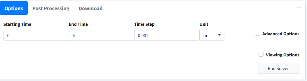
Navigate to the “Execute Model” tab on the lefthand tabbar. This tab solves our model and provides us with the options to customize the solver. For this model, we will just solve using the standard options:
Enter the following times: Starting = 0, End = 5, Step = 0.001, Unit = hr. This generates the model to be solved and integrated at time points 0, 0.001, 0.002…..5.998, 5.999, 6.
Press the “Run Solver” button.
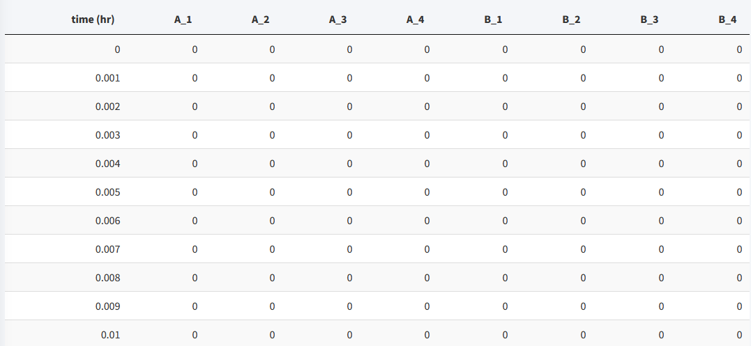
An output table should be generated with the concentration of each species along each time step of the solved model.
You can download this solved model data to a csv file in the download tab on this page. Post processing is not used in this tutorial.
Note
BioModME is set by default to show the results table rounded to 3 digits. Most terms in these results at the beginning will round to 0. To change this, check the Viewing Options box and turn off the Round option or turn on the Scientific Notation option.
Below is how the table for this model should look after the initial solve:
To see the values for the model in a good form, we will change the viewing options:
Click the Viewing Options Checkbox.
Change Results Units to umol.

In this section, we will examine the plotting of this model.
Visualization
Move to the Visualization tab. The starting plot from the model should look like the following:

For this problem we want to examine how the concentration of A varies throughout the bloodsteam (A_1, A_2, A_4). Click the Variable dropdown and remove all necessary variables:
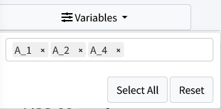
The resulting plot should look like:
